

Introduction
The promise of agentic AI—systems capable of autonomous reasoning, multi-step planning, tool execution, and self-correction—has historically been bound to massive, cloud-hosted foundation models. While cloud APIs offer vast computational scale, they introduce significant friction for enterprise applications: network latency, high operational costs, data privacy risks, and a complete reliance on persistent connectivity. For applications running on edge devices, industrial gateways, or local developer workstations, cloud-dependent agents are often non-viable.
Meta’s release of the Muse Glimmer 30B model family alongside the mature ExecuTorch runtime represents a major shift in this landscape. Muse Glimmer 30B is an open-weight model engineered specifically for local, agentic workflows. When paired with ExecuTorch—Meta’s highly modular, lightweight runtime designed for mobile and edge platforms—it becomes possible to execute complex, multi-turn tool-calling loops directly on consumer-grade hardware, local workstations, and high-end edge devices.
In this article, I will analyze the inner workings of the Muse Glimmer 30B architecture, dissect the compilation pipeline of ExecuTorch, and detail the optimization techniques required to deploy a 30B parameter model locally. I will also provide a concrete implementation strategy, evaluate the hardware trade-offs you must navigate, and outline actionable recommendations for engineering leaders looking to build offline-first agentic systems.
Architectural Breakdown: Muse Glimmer 30B and On-Device Agentic Capabilities
To understand why Muse Glimmer 30B is highly suited for local agentic tasks, we must look beyond its parameter count to its structural design. A standard 30-billion-parameter model typically presents a severe memory bottleneck for edge devices. However, Muse Glimmer 30B employs several structural optimizations designed to balance representation capacity with runtime efficiency.
Grouped-Query Attention (GQA) and Context Windows
Muse Glimmer utilizes Grouped-Query Attention (GQA) with an 8-key-value (KV) head configuration. By sharing KV heads across query heads, the model dramatically reduces the memory footprint of the KV cache during inference. This is critical for agentic workflows, which naturally demand long context windows to store system prompts, available tool definitions, historical execution traces, and retrieved documents. Muse Glimmer supports an active context window of up to 32,768 tokens. Without GQA, the KV cache for a 32k context on a 30B model would easily saturate the unified memory of high-end laptops or edge NPUs, leaving no room for the model weights themselves.
Native Tool Calling and Function Routing
Unlike general-purpose models that require complex, fragile system prompting to output structured JSON for tool execution, Muse Glimmer 30B was pre-trained and fine-tuned on synthetic and real-world execution traces. It features native, low-latency token sequences specifically reserved for tool invocation and response parsing.
When the model decides to call an external API or local system function, it emits a dedicated control token, <|start_call|>, followed by the function name and arguments in a highly compressed, deterministic format. It then pauses generation and yields control back to the runtime environment via a <|wait_response|> token. This native integration reduces parsing errors, minimizes the prompt overhead typically associated with JSON schemas, and shortens the overall planning latency.
The On-Device Agentic Loop
In a typical cloud-based agentic architecture, the loop consists of:
- User Input -> 2. Cloud LLM -> 3. JSON Parse -> 4. Local/Cloud Tool Execution -> 5. Format Results -> 6. Cloud LLM -> 7. Final Response.
On-device, this loop must be highly optimized to avoid CPU-to-GPU memory copying overhead. By running Muse Glimmer 30B within a unified memory architecture (such as Apple Silicon or modern APUs with shared system memory), the runtime can execute local system tools (e.g., querying a local SQLite database, reading sensor data, or interacting with the local file system) and feed the results back into the model's KV cache without crossing network boundaries or executing expensive serialization steps. This localized loop reduces the latency of a single agentic turn from seconds to milliseconds.
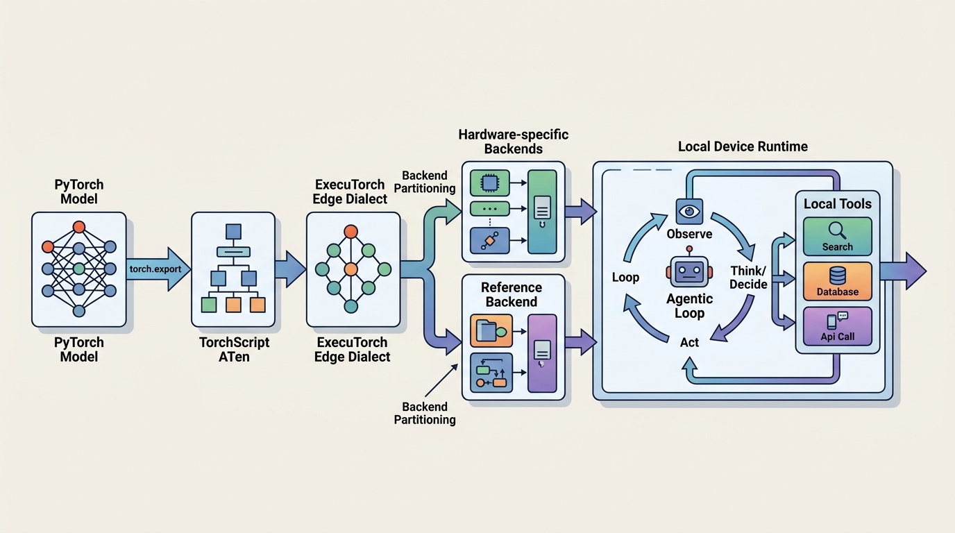
The ExecuTorch Compilation Pipeline: From PyTorch to Edge Hardware
ExecuTorch is not merely another inference engine; it is a highly specialized, end-to-end compilation and runtime framework designed to bridge the gap between PyTorch's dynamic research environment and the highly constrained, static execution environments of edge hardware.
Deploying Muse Glimmer 30B via ExecuTorch requires compiling the PyTorch model through a multi-stage pipeline. Understanding this pipeline is essential for debugging performance bottlenecks and ensuring mathematical correctness after quantization.
1. Program Capture and Export
The process begins by capturing the PyTorch model using torch.export. Unlike the older TorchScript, which relied on abstract syntax tree (AST) parsing, torch.export performs sound, graph-level tracing. It produces a clean, strongly typed computation graph represented in PyTorch's Core ATen operator set. This step eliminates Python runtime dependencies, converting dynamic control flows into static, compiled subgraphs where possible.
2. Lowering to the Edge Dialect
Once exported, the graph is lowered into the ExecuTorch "Edge Dialect." During this phase, high-level ATen operators are mapped to a restricted, highly optimized set of edge-focused operators. This is also where memory planning occurs. The ExecuTorch compiler analyzes the lifetime of every tensor in the graph and generates a static memory plan. Instead of dynamically allocating and freeing memory during inference—which leads to fragmentation and unpredictable latencies—ExecuTorch calculates the exact size of the required working memory buffer (the "arena") ahead of time. This buffer is allocated once at application startup.
3. Backend Delegation
For a 30B model, executing entirely on a mobile or edge CPU is impractical. The compilation pipeline must delegate specific subgraphs to specialized hardware accelerators, such as Apple's Neural Engine (ANE) via CoreML, Qualcomm's Hexagon NPU via the QNN delegate, or desktop GPUs via the Vulkan/MPS delegates.
During compilation, the ExecuTorch compiler partitions the graph. Operators supported by the target accelerator are grouped and compiled into a backend-specific binary payload (a "delegate blob"). The remaining unsupported operators fall back to ExecuTorch’s highly optimized reference kernels running on the CPU. This hybrid execution model ensures that you get maximum hardware acceleration without sacrificing model compatibility.
4. Serialization to .pte Format
Finally, the optimized graph, static memory plan, and compiled delegate blobs are serialized into a single flatbuffer file with the .pte extension. This file can be loaded directly by the ExecuTorch C++ runtime with minimal parsing overhead, enabling near-instantaneous application startup times.
Quantization, Memory Optimization, and Hardware Delegation
Deploying a 30B parameter model on consumer devices requires aggressive optimization. Unquantized, a 30B model in FP16 precision requires approximately 60 GB of VRAM just to load the weights, completely ruling out standard consumer laptops, mobile devices, and edge gateways. To make Muse Glimmer 30B viable, we must implement advanced quantization and memory management strategies.
Quantization Strategies: 4-bit Weight-Only vs. 8-bit Mixed Precision
To fit the model into consumer-accessible memory footprints, I recommend utilizing Post-Training Quantization (PTQ) to compress the weights.
- INT4 Weight-Only Quantization (Group-wise): By quantizing the weights to 4-bit integers while keeping the activations in FP16, we compress the model size from 60 GB to approximately 15 GB to 18 GB (depending on the grouping size, such as group-size 32 or 128). This allows the model to fit comfortably within the unified memory of a 24 GB or 32 GB RAM device, leaving sufficient headroom for the operating system and the KV cache.
- INT8 Activation Quantization: While 4-bit weight-only quantization drastically reduces storage and memory footprint, the hardware must dequantize the weights back to FP16 on-the-fly during matrix multiplication. If the target hardware's NPU supports native INT8/INT4 mixed-precision execution, quantizing both weights and activations to INT8 (or using a mixed INT4/INT8 scheme) can bypass this dequantization overhead, yielding significantly higher token-generation throughput at the cost of a minor reduction in reasoning accuracy.
Mitigating Memory Bandwidth Bottlenecks
In on-device LLM inference, the primary bottleneck is almost always memory bandwidth, not compute capability. Generating a single token requires reading the entire model's weights from memory to the processor's registers. For a compressed 15 GB model, achieving a generation speed of 15 tokens per second requires a memory bandwidth of at least 225 GB/s ($15 \text{ GB} \times 15 \text{ tokens/sec}$).
This reality dictates my hardware recommendations: you should target platforms with high-bandwidth unified memory architectures (such as Apple Silicon Pro/Max chips with 150–400 GB/s bandwidth, or specialized edge modules like the NVIDIA Jetson AGX Orin with 2048-bit memory interfaces yielding 275 GB/s). Standard x86 laptops with dual-channel DDR5 memory (typically limited to 60–80 GB/s) will struggle to exceed 4 to 5 tokens per second with a 30B model, which may be too slow for highly interactive agentic loops but remains acceptable for background processing tasks.
ExecuTorch Memory Arenas and Zero-Copy Loading
To prevent the operating system from killing your application due to sudden memory spikes, ExecuTorch allows you to manage memory explicitly. By utilizing zero-copy memory mapping (mmap), the C++ runtime can map the .pte model file directly from storage into the virtual address space. This avoids copying the model weights into RAM twice. Combined with the pre-allocated execution arena, the memory footprint of your agentic application remains completely flat and predictable throughout its execution life cycle.
Implementing an On-Device Agentic Loop: Code and Execution
The following Python script demonstrates how to export the Muse Glimmer 30B model, apply 4-bit group-wise quantization, and compile it into an ExecuTorch .pte program optimized for an MPS (Metal Performance Shaders) backend. This represents the compilation phase that occurs on your development machine before deploying the artifact to the target edge device.
import torch
from torch.export import export
from executorch.exir import EdgeCompileConfig, to_edge
from executorch.backends.apple.mps.compiler import mps_to_backend
from executorch.extension.llm.quantizer import Quantizer, WeightOnlyInt4Quantizer

# 1. Initialize the Muse Glimmer 30B Model (Stubbed for compilation demonstration)
class MuseGlimmer30BStub(torch.nn.Module):
    def __init__(self):
        super().__init__()
        # In production, this would load the actual model architecture
        self.token_embeddings = torch.nn.Embedding(32000, 7168)
        self.output_projection = torch.nn.Linear(7168, 32000, bias=False)

    def forward(self, tokens: torch.Tensor, input_pos: torch.Tensor) -> torch.Tensor:
        x = self.token_embeddings(tokens)
        # Simulate a simplified transformer layer pass
        x = x + torch.ones_like(x) * 0.01
        logits = self.output_projection(x)
        return logits

model = MuseGlimmer30BStub().eval()

# Create representative inputs for tracing (batch_size=1, sequence_length=512)
example_tokens = torch.randint(0, 32000, (1, 512), dtype=torch.long)
example_pos = torch.arange(0, 512, dtype=torch.long)
example_inputs = (example_tokens, example_pos)

# 2. Export the PyTorch model to a clean ATen Graph
print("[INFO] Exporting model to ATen Graph...")
with torch.no_grad():
    exported_program = export(model, example_inputs)

# 3. Apply Weight-Only 4-bit Quantization
print("[INFO] Applying 4-bit group-wise quantization...")
quantizer = WeightOnlyInt4Quantizer(groupsize=128)
# In a real pipeline, you would register the quantizer to target specific linear layers
# e.g., quantizer.register_block_filter(lambda node: "output_projection" in node.name)

# 4. Lower to ExecuTorch Edge Dialect
print("[INFO] Lowering to ExecuTorch Edge Dialect...")
edge_config = EdgeCompileConfig(_use_aten_decomposition=True)
edge_program = to_edge(exported_program, compile_config=edge_config)

# 5. Delegate to MPS (Metal Performance Shaders) for Apple Silicon Acceleration
print("[INFO] Partitioning and delegating to MPS backend...")
# The compiler identifies subgraphs compatible with MPS and compiles them
mps_edge_program = edge_program.to_backend(mps_to_backend)

# 6. Serialize the final optimized program to a .pte file
output_path = "muse_glimmer_30b_mps.pte"
print(f"[INFO] Serializing program to {output_path}...")
with open(output_path, "wb") as f:
    f.write(mps_edge_program.buffer())

print("[SUCCESS] Compilation complete. Ready for on-device deployment.")
Once compiled, this .pte file is loaded by your on-device C++ application. The application wraps the ExecuTorch runtime and drives the agentic loop. When the model outputs a tool call, your application intercepts the token stream, executes the requested system command, formats the output, and appends it back to the input tensor sequence for the next forward pass.
Operational Trade-Offs and Engineering Recommendations
Deploying a 30B parameter model at the edge requires making deliberate trade-offs between performance, accuracy, and hardware costs. The following table outlines the performance profiles across typical target deployment environments to help you make informed architectural decisions.
| Target Hardware Platform | Memory Bandwidth | Quantization Level | Expected Latency (Tokens/Sec) | Primary Operational Trade-off | Recommended Use Case |
|---|---|---|---|---|---|
| High-End Workstation (e.g., Apple M3 Max 128GB Unified RAM) | ~400 GB/s | INT4 Weight-Only | 22 - 28 t/s | High hardware unit cost; excellent local performance and zero thermal throttling. | Local developer environments, high-priority offline workstations. |
| Industrial Edge Gateway (e.g., NVIDIA Jetson AGX Orin 64GB) | ~275 GB/s | INT8 Mixed-Precision | 12 - 18 t/s | High power consumption (up to 60W); requires active cooling solutions. | Smart factories, local robotics controllers, on-premise secure gateways. |
| Standard Enterprise Laptop (e.g., Intel Core Ultra / AMD Ryzen 9, 32GB LPDDR5) | ~75 GB/s | INT4 Weight-Only | 4 - 6 t/s | Low token throughput; high battery drain during sustained agentic loops. | Occasional offline productivity assistants, asynchronous background agents. |
| Mobile Edge Devices (e.g., High-End Tablets / Smartphones, 16GB RAM) | ~100 GB/s | INT3/INT4 Mixed | 2 - 4 t/s | Extreme memory pressure; high risk of OS-level process termination. | Highly constrained, localized field diagnostics with small context windows. |
Strategic Recommendations for Engineering Leaders
If you are evaluating whether to deploy on-device agentic architectures using Muse Glimmer 30B and ExecuTorch, I recommend the following phased approach:
- Establish a Strict Memory Budget: Before writing any code, define your target hardware's hard memory limit. For a 32 GB RAM target device, allocate a maximum of 16 GB for the model weights, 4 GB for the active KV cache (which scales linearly with context length), and 2 GB for the ExecuTorch runtime execution arena. This leaves 10 GB for the operating system and host application, preventing Out-Of-Memory (OOM) crashes.
- Implement Fallback Strategies for Tool Failures: Unlike cloud environments where tool execution environments can be easily sandboxed and scaled, on-device tool execution interacts directly with physical hardware and local files. Your wrapper application must implement strict sandboxing, timeout limits, and robust exception handling to ensure that a failing local tool does not crash the entire agentic loop.
- Optimize the KV Cache Dynamically: Since agentic loops can run for many turns, the KV cache will grow rapidly. Implement KV cache eviction policies (such as sliding window attention or heavy-hitter eviction) within your ExecuTorch runtime wrapper to keep the memory footprint stable during long-running sessions.
- Validate Quantization Loss with Task-Specific Benchmarks: Quantizing a model to 4-bit can occasionally degrade its reasoning capabilities or cause it to hallucinate tool arguments. Create a regression test suite consisting of 50 to 100 deterministic tool-calling scenarios. Run this suite against both the unquantized FP16 model and your compiled
.ptemodel to quantify the exact impact of quantization on your specific domain before shipping to production.
Conclusion
The combination of Meta's Muse Glimmer 30B and the ExecuTorch runtime represents a significant milestone for edge computing and local AI. By moving the agentic loop entirely on-device, you eliminate network latency, guarantee data privacy, and slash cloud API costs.
However, achieving production-grade performance requires a deep understanding of hardware constraints, compilation pipelines, and memory optimization. By carefully quantizing your models, leveraging hardware-specific delegates, and maintaining strict control over your memory footprint, you can build resilient, highly responsive, and completely offline agentic systems that operate reliably in any environment.